The goal of resourcecode is to provide an easy access to the ResourceCODE hindcast database of sea-states. More information on the database can be found here. We will explain in this vignette the way to retrieve data from this database and some the functionalities offered by this package.
Once the packages are installed, we can proceed as usual:
Database configuration: nodes, bathymetry…
There are two grids in the ResourceCODE hindcast database: the full, dense, FIELD grid, which is the grid where the numerical WWIII model is run and where sea-state parameters and only 1D spectra are available. The second grid, SPEC, is coarser, but contains the full 2D spectral data at each node.
- FIELD grid
The variable rscd_field contains the coordinates of the
FIELD grid, along with the depth of these points and d50,
the bottom sediment type.
str(rscd_field)
#> 'data.frame':    328030 obs. of  5 variables:
#>  $ node     : int  1 2 3 4 5 6 7 8 9 10 ...
#>  $ longitude: num  6.92 6.91 6.92 6.93 6.95 ...
#>  $ latitude : num  62.9 62.9 62.9 62.9 62.9 ...
#>  $ depth    : num  3 3 3 3 3 3 3 3 3 3 ...
#>  $ d50      : num  0 1.32 1.32 1.32 1.32 ...
head(rscd_field)
#>   node longitude latitude depth   d50
#> 1    1  6.922498 62.91467     3 0.000
#> 2    2  6.910178 62.91301     3 1.322
#> 3    3  6.920552 62.90438     3 1.322
#> 4    4  6.933673 62.89938     3 1.322
#> 5    5  6.945979 62.90012     3 1.322
#> 6    6  6.958059 62.89899     3 1.322
At each location, a large number of sea-state parameters are
available, described in rscd_variables:
str(rscd_variables)
#> 'data.frame':    88 obs. of  3 variables:
#>  $ name    : chr  "longitude" "latitude" "tri" "MAPSTA" ...
#>  $ longname: chr  "longitude" "latitude" "tri" "status map" ...
#>  $ unit    : chr  "degree_east" "degree_north" "" "1" ...
head(rscd_variables)
#>        name         longname         unit
#> 1 longitude        longitude  degree_east
#> 2  latitude         latitude degree_north
#> 3       tri              tri
#> 4    MAPSTA       status map            1
#> 5       dpt            depth            m
#> 6      ucur eastward current        m s-1
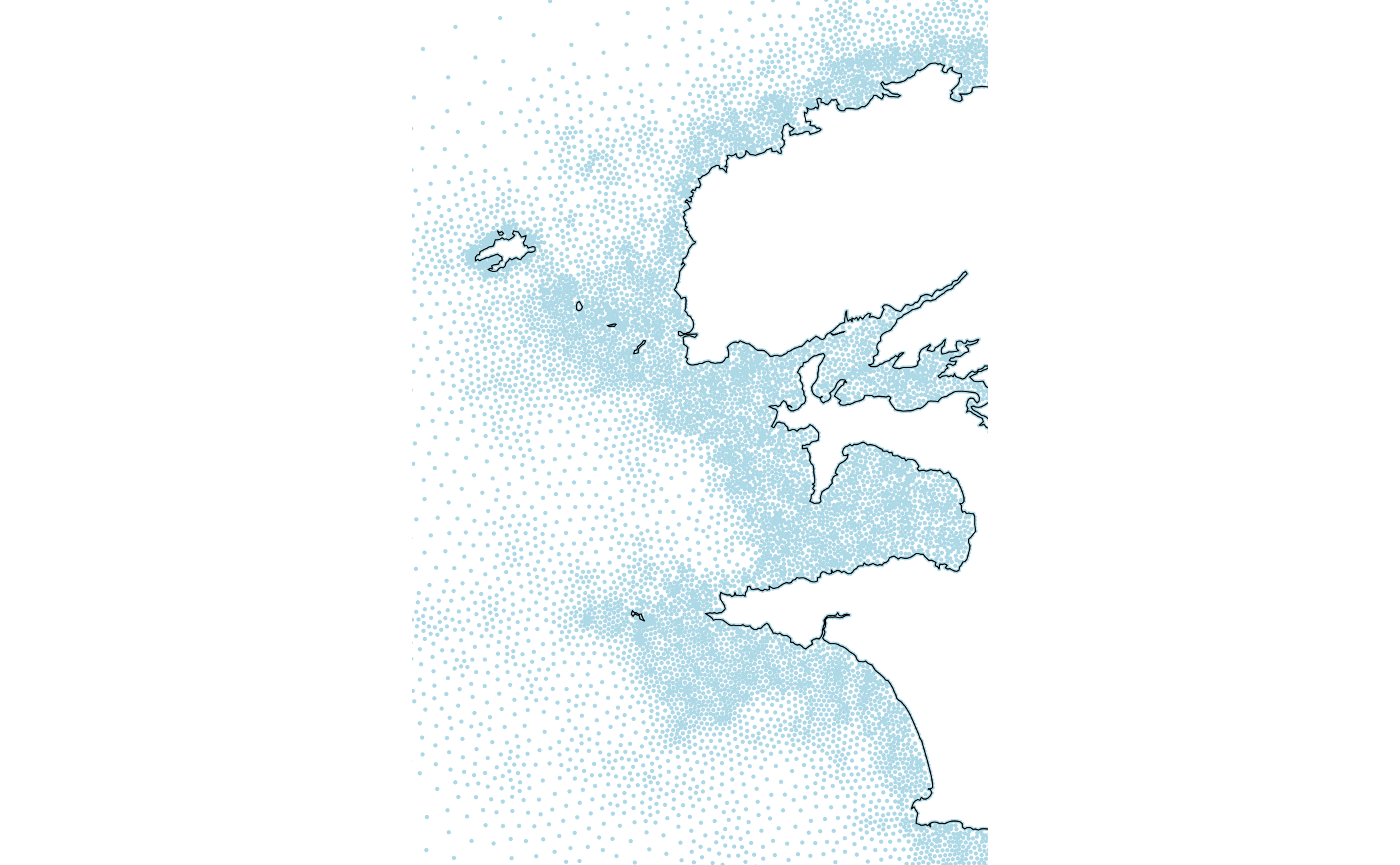
The available location can be plotted on a map using the following
code. It can be noticed here that the variables
rscd_coastline and rscd_islands contain the
path of the coast line and the islands, respectively.
lim_lon <- c(-5.25, -4.25)
lim_lat <- c(47.75, 48.75)
field_bzh <- ggplot(rscd_field, aes(x = longitude, y = latitude)) +
  geom_point(size = .1, col = "lightblue") +
  geom_path(data = rscd_coastline, linewidth = .2) +
  geom_path(data = rscd_islands, aes(group = .data$ID), linewidth = .2) +
  coord_sf(xlim = lim_lon, ylim = lim_lat, expand = FALSE, crs = sf::st_crs(4326)) +
  theme_void()
field_bzh
- SPEC grid
The spectral grid, or SPEC grid is coarser, with more than 24,000 nodes where the full 2D spectra are available. The grid can be added to the previous plot to see the differences in the spatial coverage.
str(rscd_spectral)
#> 'data.frame':    24276 obs. of  5 variables:
#>  $ longitude: num  1.5 -5.5 -6 -6.5 -7 4.5 4 3.5 3 2.5 ...
#>  $ latitude : num  52 52 52 52 52 52.5 52.5 52.5 52.5 52.5 ...
#>  $ name     : chr  "E001500N52000" "W005500N52000" "W006000N52000" "W006500N52000" ...
#>  $ depth    : num  15.4 89.6 95.8 52.7 54.7 ...
#>  $ d50      : num  0.737 -0.8265 -1.585 0.737 0.0346 ...
head(rscd_spectral)
#>   longitude latitude          name    depth         d50
#> 1       1.5     52.0 E001500N52000 15.41327  0.73700004
#> 2      -5.5     52.0 W005500N52000 89.64895 -0.82650555
#> 3      -6.0     52.0 W006000N52000 95.83614 -1.58500008
#> 4      -6.5     52.0 W006500N52000 52.67409  0.73700004
#> 5      -7.0     52.0 W007000N52000 54.67464  0.03464983
#> 6       4.5     52.5 E004500N52500 14.18527  0.73700004
field_bzh + geom_point(data = rscd_spectral, col = "orange", size = .1)
- Helpers to find points
When one is interested in some location, we also provide helpers to
find the closest point in each of the grid, via the
closest_point_FIELD() and closest_point_SPEC()
functions.
Getting data
We have two different sources of data, the FIELD grid, and the SPEC grid. We will cover each use case here.
- Sea-state parameters from the FIELD can be retrieved using the
get_parameters()function, which allows to download a time series easily at a given location. For the moment (Sept. 2023), the 1D spectra on this grid are not available to direct download.
For example, if one is interested in the time series of sea-state parameters at some location, the following code can be adapted:
point_of_interest <- c(longitude = -4.6861533, latitude = 48.3026514)
node <- closest_point_field(point_of_interest)
node
#> $points
#>        [,1]
#> [1,] 134940
#>
#> $distances
#>         [,1]
#> [1,] 288.974
ts <- get_parameters(node = node$point, parameters = c("hs", "tp", "dp", "cge"))
if (!is.null(ts)) {
  ggplot(tidyr::pivot_longer(ts, -1), aes(x = time, y = value, col = name)) +
    geom_line() +
    coord_cartesian(expand = FALSE) +
    facet_wrap(~name, ncol = 2, scales = "free_y") +
    scale_x_datetime(name = NULL, date_breaks = "month") +
    scale_y_continuous(name = NULL) +
    theme_minimal() +
    theme(
      legend.position = "none",
      axis.text.x = element_text(angle = 60, hjust = 1)
    )
}
- 1D and 2D spectra of the SPEC grid can be downloaded directly from
IFREMER FTP using functions
get_1Dspectrum()andget_2Dspectrum(). We also provide a plotting function for the 2D spectrum.
node_spectral_grid <- closest_point_spec(point_of_interest)Then one can extract the 1D spectrum time-series and see the contents of these downloaded data.
spec_1d <- get_1d_spectrum(node_spectral_grid$point, start = "1994-01-01", end = "1994-02-28")
str(spec_1d)
We also provide in the package resourcecodedata pre-loaded time series of 1D spectra, mainly for testing and example purpose:
spec_1d <- resourcecodedata::rscd_1d_spectra
str(spec_1d)
The same applies to 2D spectra:
spec_2d <- get_2d_spectrum(node_spectral_grid$point, start = "1994-01-01", end = "1994-02-28")
str(resourcecodedata::rscd_2d_spectra)
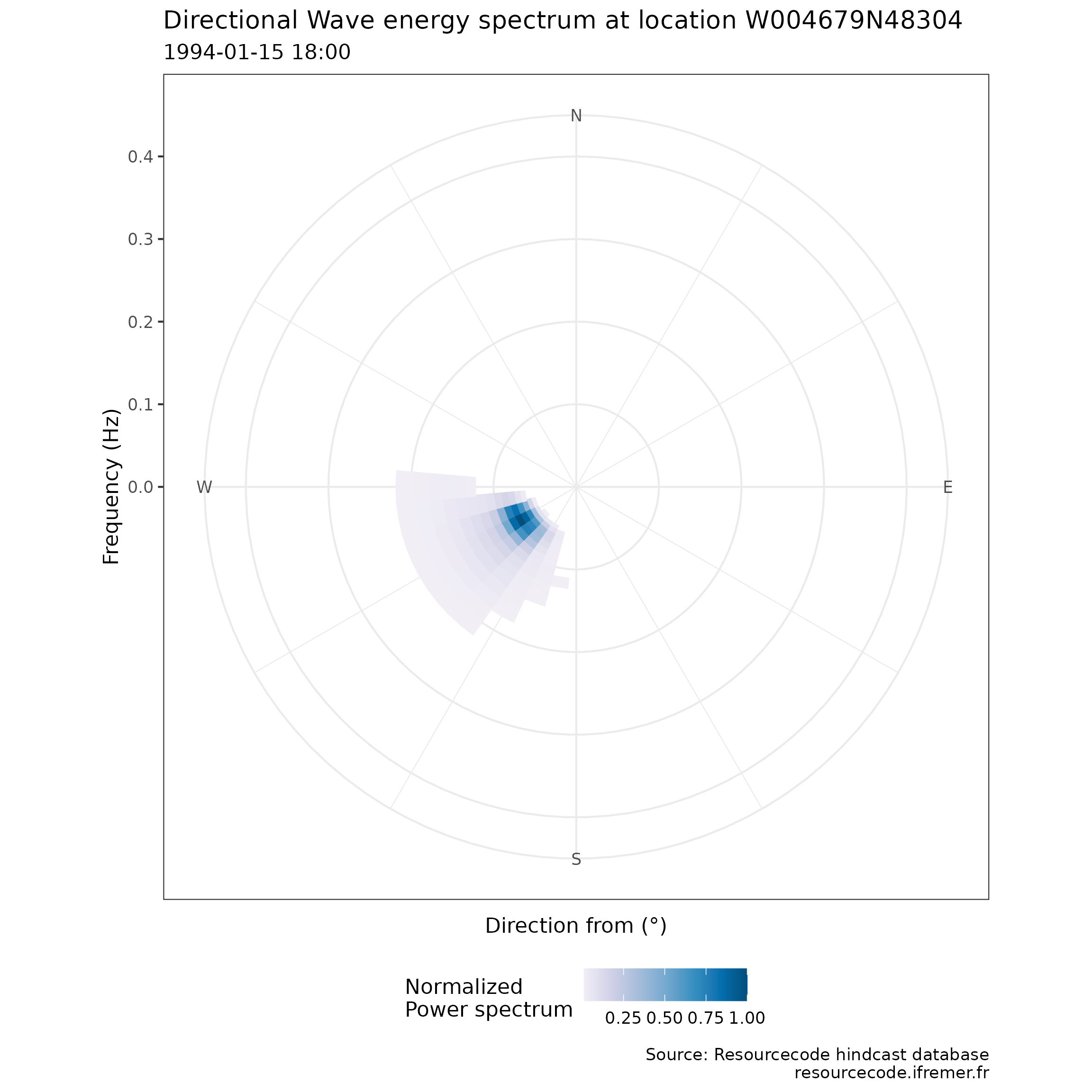
In addition, it is possible to plot the wave elevation directional spectra for any given time, which can be specified by the time index or directly the date:
plot_2d_specta(resourcecodedata::rscd_2d_spectra, "1994-01-15 18:00")
