Estimation of producible energy

In this example, we will estimate WEC energy production using the ResourceCode hindcast data as an input and capture width data of a standard WEC to simulate the behaviour and estimate energy that can be harvested with this device from the slected location.

See also

In addition, a demonstration tool based on this module can be accessed on the Resourcecode Tools web page.

import pandas as pd
import numpy as np
from pathlib import Path
import matplotlib.pyplot as plt
import resourcecode
from resourcecode import producible_assessment
from resourcecode.spectrum import compute_jonswap_wave_spectrum
import warnings

warnings.filterwarnings("ignore")
plt.rcParams["figure.dpi"] = 400
# sphinx_gallery_thumbnail_number = 2

Load WEC characteristics: PTO, capture width and corresponding frequencies

Default characteristics are provided with the package, but the user is free to change it to use a specific device.

DATA_DIR = Path(producible_assessment.__file__).parent / "Inputs"
capture_width = pd.read_csv(DATA_DIR / "capture_width.csv", delimiter=",", header=None)
freq = pd.read_csv(DATA_DIR / "Frequencies.csv", delimiter=",", header=None)
pto_data = pd.read_csv(DATA_DIR / "PTO_values.csv", delimiter=",", header=None)
capture_width.columns = pto_data.values.tolist()[0]
capture_width.index = [val for sublist in freq.values.tolist() for val in sublist]

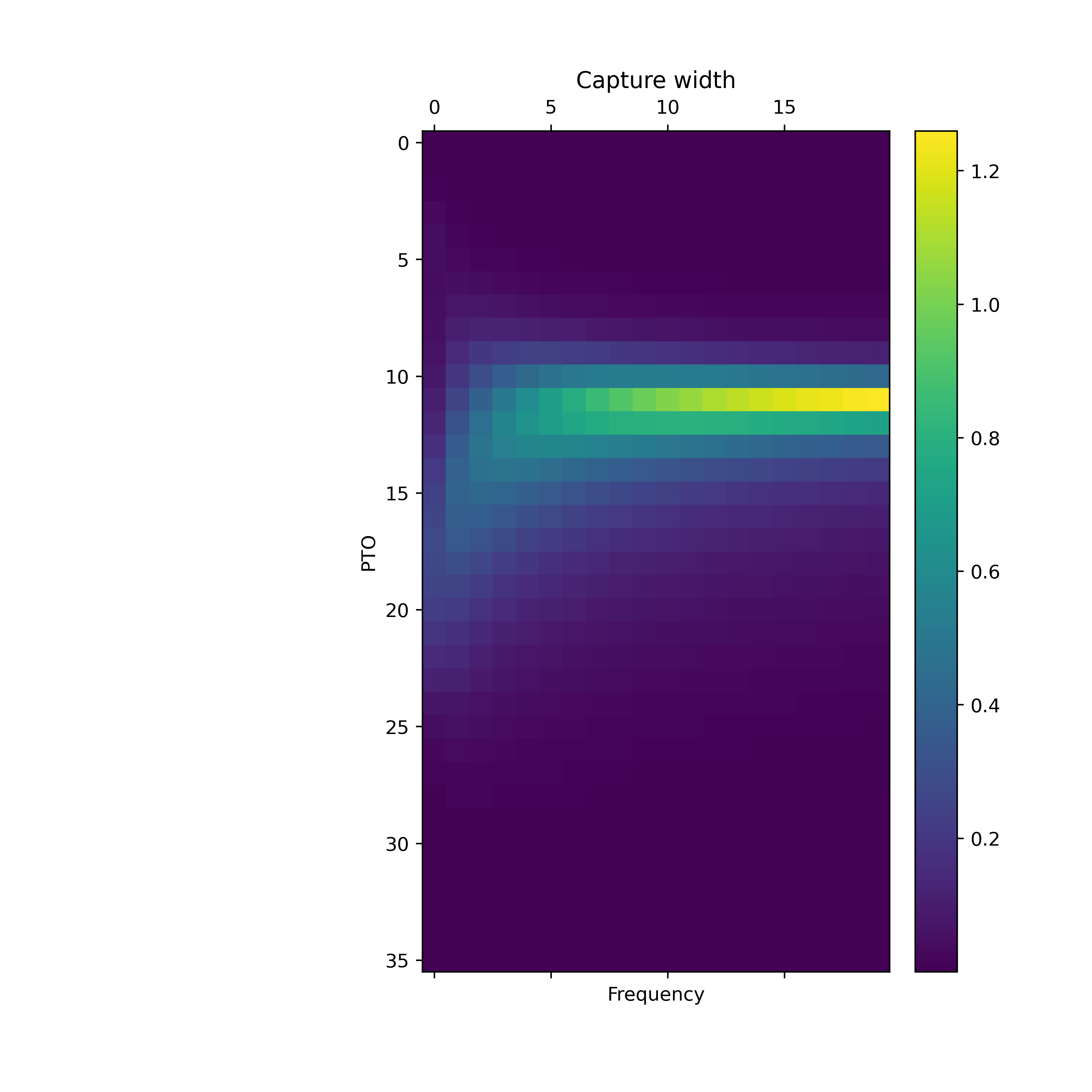
Plot of the characteristics of the WEC

fig = plt.figure(figsize=(8, 8))
ax = plt.gca()
plt.xlabel("Frequency")
plt.ylabel("PTO")
img = ax.matshow(capture_width.to_numpy())
fig.colorbar(img, fraction=0.08, pad=0.03)
plt.title("Capture width")
plt.show()

We then extract the time series of 1D wave spectra from the RESOURCECODE database, using the resourcecode.spectrum.download_data.get_1D_spectrum() function. For this example, we used the data from the SEMREVO location. We only need the frequency spectrum in this case, so we convert it to a pandas DataFrame.

spec1D = resourcecode.spectrum.download_data.get_1D_spectrum(
    "SEMREVO", ["2014"], ["02"]
)
spec = spec1D.ef.to_pandas()

# The frequency has been truncated, so here we reconcile both
spec.columns = capture_width.index

We propose here to compare with the PTO estimated using a JONSWAP approximation, so we need the sea-state parameters data to compute the JONSWAP spectrum.

client = resourcecode.Client()
wave_data = client.get_dataframe(
    pointId=119947,
    startDateTime="2014-02-01T00:00:00",
    endDateTime="2014-02-28T23:00:00",
    parameters=("hs", "tp"),
)

freq_vec = capture_width.index
jonswap = compute_jonswap_wave_spectrum(wave_data, freq_vec)

Once the spectral data is available, one can estimate the Power Take-off (PTO) of the WEC.

pto_jonswap = producible_assessment.PTO(capture_width, jonswap)
pto = producible_assessment.PTO(capture_width, spec)

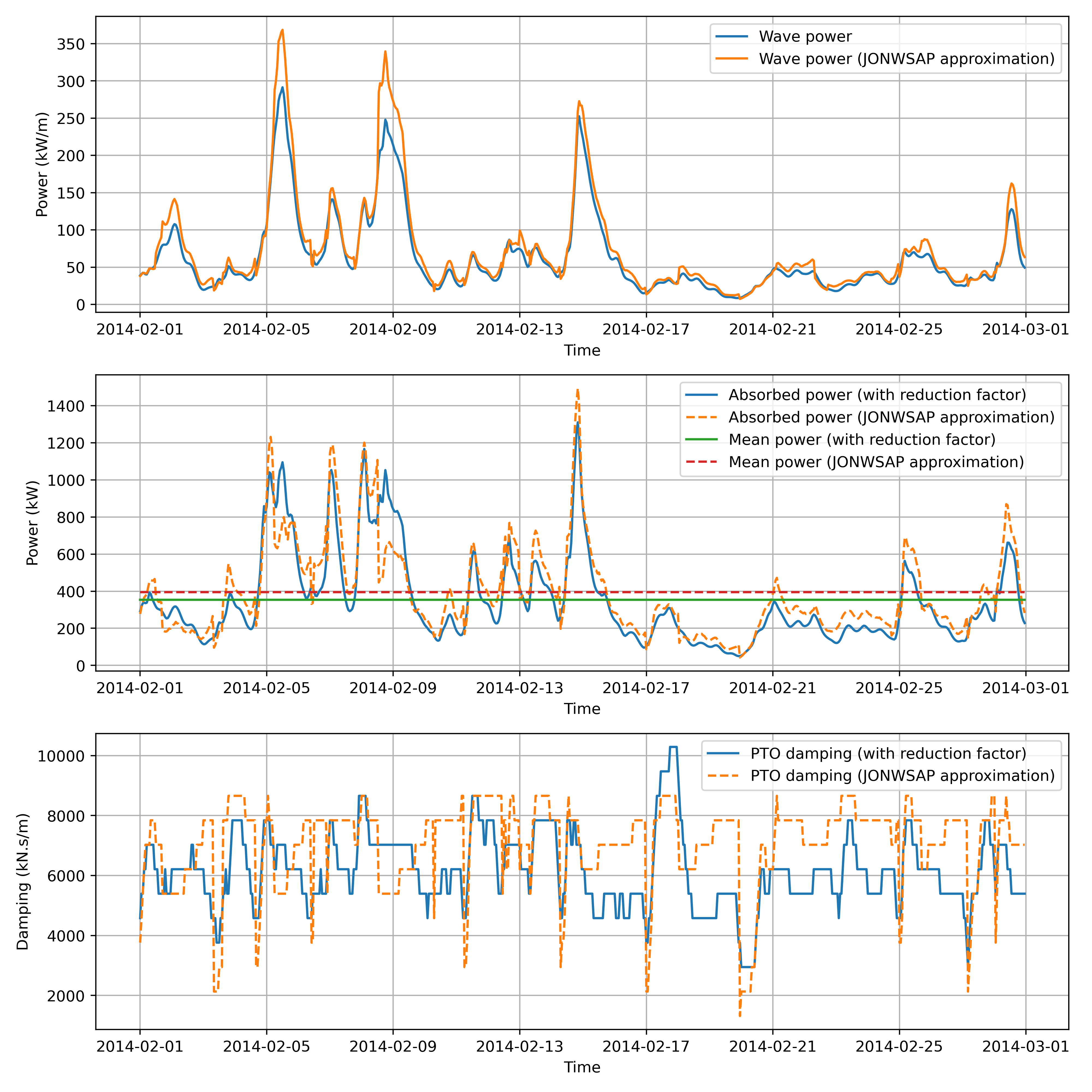
Plot PTO results time series in 3 subplots where we can compare the estimation with or without the JONSWAP approximation: wave power, absorbed/mean power with reduction factor, PTO damping with reduction factor. Power is converted from W to kW, damping from Ns/m to kNs/m.

# plot wave power
fig, (ax1, ax2, ax3) = plt.subplots(3, 1, figsize=(10, 10))
ax1.plot(pto.wave_power.div(1000 * pto.width))
ax1.plot(pto_jonswap.wave_power.div(1000 * pto_jonswap.width))
ax1.legend(["Wave power", "Wave power (JONWSAP approximation)"])
ax1.grid()
ax1.set(xlabel="Time", ylabel="Power (kW/m)")
# absorbed/mean power
all_time_series = [
    pto.power,
    pto_jonswap.power,
    pto.mean_power,
    pto_jonswap.mean_power,
]
linestyles = ["solid", "dashed", "solid", "dashed"]
for time_series, linestyle in zip(all_time_series, linestyles):
    ax2.plot(time_series.div(1000), linestyle=linestyle)
ax2.legend(
    [
        "Absorbed power (with reduction factor)",
        "Absorbed power (JONWSAP approximation)",
        "Mean power (with reduction factor)",
        "Mean power (JONWSAP approximation)",
    ]
)
ax2.grid()
ax2.set(xlabel="Time", ylabel="Power (kW)")
# PTO damping
all_time_series = [pto.pto_damp, pto_jonswap.pto_damp]
for time_series, linestyle in zip(all_time_series, linestyles):
    ax3.plot(time_series.div(1000), linestyle=linestyle)
ax3.legend(
    [
        "PTO damping (with reduction factor)",
        "PTO damping (JONWSAP approximation)",
    ]
)
ax3.grid()
ax3.set(xlabel="Time", ylabel="Damping (kN.s/m)")
plt.tight_layout()

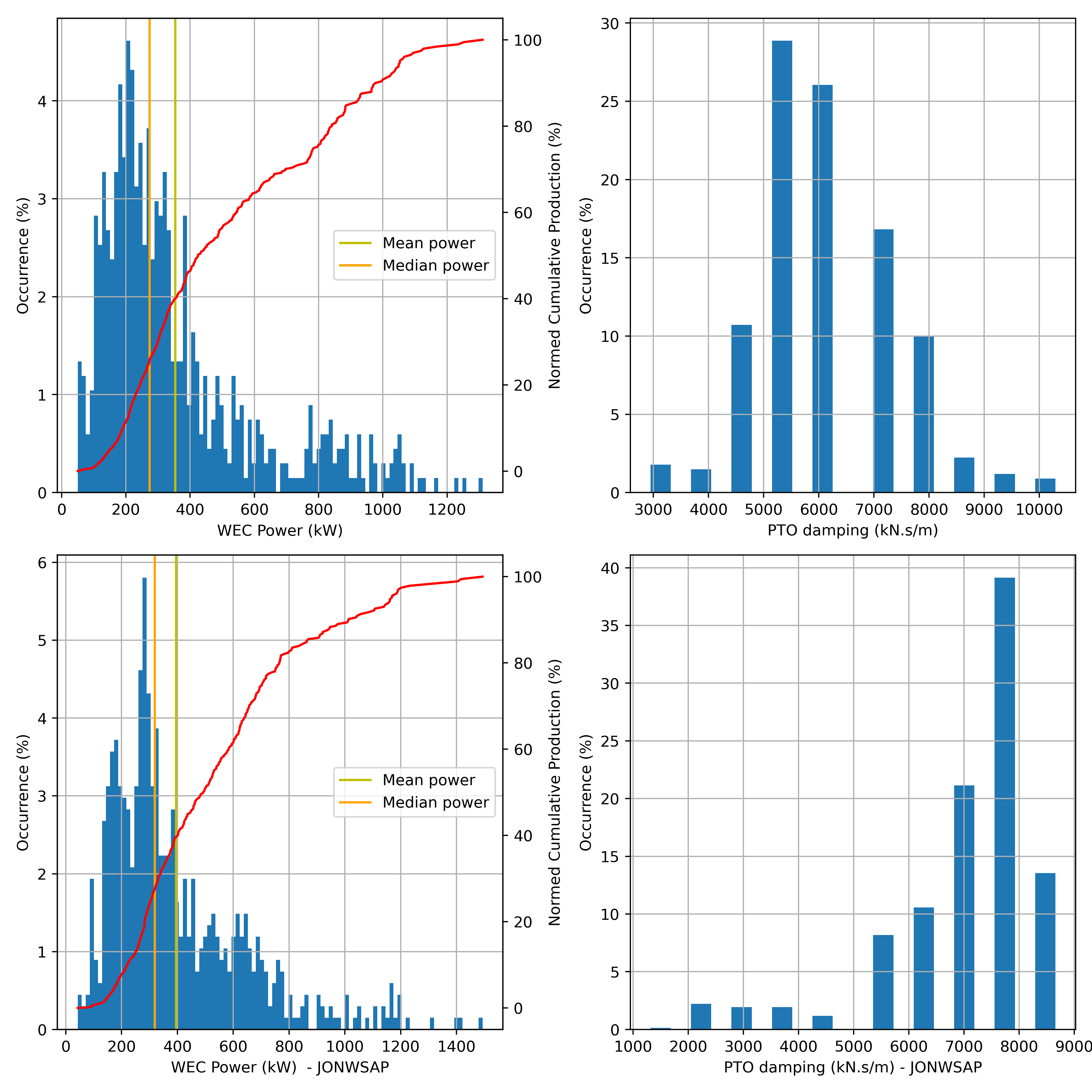
The plots below show the repartition of WEC power in the two cases considered and the histogram of corresponding damping.

fig, ((ax1, ax2), (ax3, ax4)) = plt.subplots(2, 2, figsize=(10, 10))
# absorbed power
power_kw = pto.power.div(1000)
# cumulative power
cumulative_power_kw = pto.cumulative_power
power_ordered = pto.power.sort_values(by=0)
index = [x / 1000 for x in power_ordered[0]]
cumulative_power_kw.index = index
# mean power
mean_power_kw = pto.mean_power[0][pto.times[0]] / 1000
# median power
median_power_kw = pto.median_power[0][pto.times[0]] / 1000
# power occurrences, cumulative power, mean and median power
ax1 = power_kw.plot.hist(
    ax=ax1,
    bins=len(pto.capture_width.columns) * 5,
    legend=False,
    weights=np.ones_like(power_kw[power_kw.columns[0]]) * 100.0 / len(power_kw),
)
ax1b = ax1.twinx()
cumulative_power_kw.plot(ax=ax1b, legend=False, color="r")
ax1.grid()
ax1.set_xlabel("WEC Power (kW)")
ax1.set_ylabel("Occurrence (%)")
ax1b.set_ylabel("Normed Cumulative Production (%)")
line_mean = ax1.axvline(x=mean_power_kw, color="y")
line_median = ax1.axvline(x=median_power_kw, color="orange")
ax1.legend([line_mean, line_median], ["Mean power", "Median power"], loc="center right")

# plot PTO histogram
pto_damp_kn = pto.pto_damp / 1000
pto_damp_kn.plot.hist(
    ax=ax2,
    bins=len(pto.capture_width.columns),
    legend=False,
    weights=np.ones_like(pto_damp_kn[pto_damp_kn.columns[0]])
    * 100.0
    / len(pto_damp_kn),
)
ax2.grid()
ax2.set_xlabel("PTO damping (kN.s/m)")
ax2.set_ylabel("Occurrence (%)")

# absorbed power (JONWSAP)
power_kw = pto_jonswap.power.div(1000)
# cumulative power
cumulative_power_kw = pto_jonswap.cumulative_power
power_ordered = pto_jonswap.power.sort_values(by=0)
index = [x / 1000 for x in power_ordered[0]]
cumulative_power_kw.index = index
# mean power
mean_power_kw = pto_jonswap.mean_power[0][pto_jonswap.times[0]] / 1000
# median power
median_power_kw = pto_jonswap.median_power[0][pto_jonswap.times[0]] / 1000
# power occurrences, cumulative power, mean and median power
ax3 = power_kw.plot.hist(
    ax=ax3,
    bins=len(pto_jonswap.capture_width.columns) * 5,
    legend=False,
    weights=np.ones_like(power_kw[power_kw.columns[0]]) * 100.0 / len(power_kw),
)
ax3b = ax3.twinx()
cumulative_power_kw.plot(ax=ax3b, legend=False, color="r")
ax3.grid()
ax3.set_xlabel("WEC Power (kW)  - JONWSAP")
ax3.set_ylabel("Occurrence (%)")
ax3b.set_ylabel("Normed Cumulative Production (%)")
line_mean = ax3.axvline(x=mean_power_kw, color="y")
line_median = ax3.axvline(x=median_power_kw, color="orange")
ax3.legend([line_mean, line_median], ["Mean power", "Median power"], loc="center right")

# plot PTO histogram
pto_damp_kn = pto_jonswap.pto_damp / 1000
pto_damp_kn.plot.hist(
    ax=ax4,
    bins=len(pto.capture_width.columns),
    legend=False,
    weights=np.ones_like(pto_damp_kn[pto_damp_kn.columns[0]])
    * 100.0
    / len(pto_damp_kn),
)
ax4.grid()
ax4.set_xlabel("PTO damping (kN.s/m) - JONWSAP")
ax4.set_ylabel("Occurrence (%)")
plt.tight_layout()