Extract some time-series from the database and analysis

import resourcecode
import resourcecode.spectrum
import matplotlib.pyplot as plot

plot.rcParams["figure.dpi"] = 400

Node selection and data extraction

Below, we will look for data next to the location of interest, located in the vicinity of Brest Bay. We will look at the time-series data and also some spectral data

selected_node = resourcecode.data.get_closest_point(
    latitude=48.3026514, longitude=-4.6861533
)
selected_node

(134940, 296.89)

selected_specPoint = resourcecode.data.get_closest_station(
    latitude=48.3026514, longitude=-4.6861533
)
selected_specPoint

('W004679N48304', 808.82)

Extraction of data from the Hindcast database

Sea-state parameters extraction and helpers from the toolbox

Once the node is selected, it is possible to retrieve the data from the Cassandra database using the commands below. It is also possible to select which variables to retrieve. The list of available variables can be obtained using the get_variables method. We study here the following variables:

• \(H_s\), the significant wave height;

• \(T_p\) the peak period;

• \(D_p\) the direction at peak frequency;

• The energy flux \(CgE\);

• zonal and meridional velocity components of wind;

For this example, we have selectedonly year 2010.

client = resourcecode.Client()
data = client.get_dataframe(
    pointId=selected_node[0],
    startDateTime="2010-01-01T01:00:00",
    endDateTime="2011-01-01T00:00:00",
    parameters=("hs", "uwnd", "vwnd", "t02", "tp", "dp", "cge"),
)
data.head()

	hs	uwnd	vwnd	t02	tp	dp	cge
2010-01-01 01:00:00	1.360	-6.0	-6.7	4.78	11.363636	221.0	9.3
2010-01-01 02:00:00	1.350	-6.0	-7.0	4.68	11.363636	221.0	8.9
2010-01-01 03:00:00	1.324	-5.6	-7.3	4.62	11.494253	222.0	8.5
2010-01-01 04:00:00	1.282	-5.4	-7.8	4.56	11.494253	223.0	7.9
2010-01-01 05:00:00	1.220	-5.3	-8.1	4.60	11.494253	224.0	7.2

With the toolbox, is is possible to convert zonal and meridional velocity components of wind the the more convenient Intensity-direction variables.

data["wspd"], data["wdir"] = resourcecode.utils.zmcomp2metconv(data.uwnd, data.vwnd)

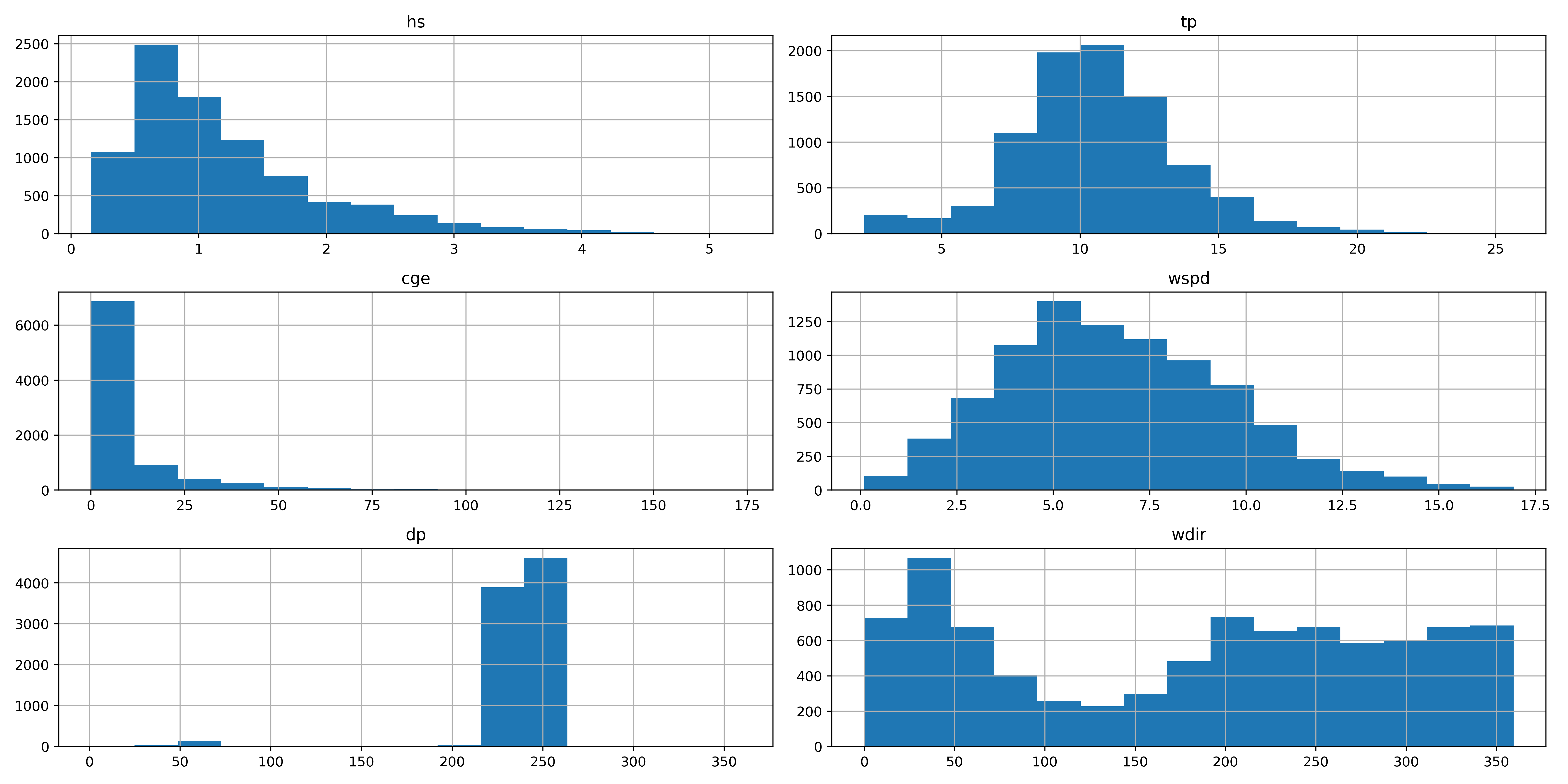
The figure below is an example of the histograme of the variables that can be extracted from the database. \(H_s\),:math:T_p, \(W_s\) and \(CgE\) are shown here with the wind and wave directions, but the code can be changed to plot any of the available variables in the Hindcast database.

data[["hs", "tp", "cge", "wspd", "dp", "wdir"]].hist(bins=15, figsize=[16, 8])
plot.tight_layout()

Spectral data extraction and computation of sea-state parameters

The toolbox also offers the possibility to download the spectral data from the coarser ‘SPEC’ grid, corresponding to the orange dots of the web portal. This is possible thanks to the get_2D_spectrum and get_1D_spectrum from the spectrum module. An example is shown below:

spec = resourcecode.spectrum.get_2D_spectrum(
    selected_specPoint[0], years=["2010"], months=["01"]
)

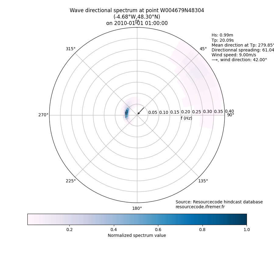
And we offer function to represent the spectral data, both for 2D and 1D spectrum.

resourcecode.spectrum.plot_2D_spectrum(spec, 1)
plot.show()

There is also function to compute the 1D spectrum from the 2D.

spec1D = resourcecode.spectrum.convert_spectrum_2Dto1D(spec)
resourcecode.spectrum.plot_1D_spectrum(spec1D, 1, sea_state=False)

<Figure size 700x500 with 1 Axes>

Among the functionalities of the toolbox, it is possible to compute the sea-state parameters from spectral data. Small discrepancies can be found between the Hindcast sea-state parameters and the one computed with the toolbox.

parameters_df = resourcecode.spectrum.compute_parameters_from_2D_spectrum(
    spec, use_depth=True
)
parameters_df.head()

	time	Hm0	Tp	T01	T02	Te	mu	nu	CgE	km	lm	depth	Thetam	Thetapm	Spr	Qp	wnd	wnddir	cur	curdir
0	2010-01-01 00:00:00	1.258713	11.382546	6.299747	4.894921	9.126643	0.629497	0.810161	8.091658	0.173012	36.316369	28.5	221.665815	221.841529	52.452013	1.905638	9.0	44.400002	0.3	218.900009
0	2010-01-01 01:00:00	1.271215	11.273698	6.118387	4.806066	8.845303	0.618847	0.787826	8.000145	0.178597	35.180836	30.0	222.276735	222.227011	55.652089	1.780164	9.0	42.000000	0.4	227.199997
0	2010-01-01 02:00:00	1.270940	11.310064	5.964570	4.717962	8.617916	0.611819	0.773477	7.790361	0.184614	34.034173	31.5	223.474217	222.590049	57.603553	1.701667	9.2	40.200001	0.3	234.600006
0	2010-01-01 03:00:00	1.250777	11.416240	5.887424	4.667331	8.503349	0.609530	0.768868	7.451620	0.188269	33.373499	32.5	226.098226	223.223522	58.092844	1.701595	9.2	37.799999	0.2	246.000000
0	2010-01-01 04:00:00	1.213452	11.484228	5.851882	4.627031	8.463007	0.612215	0.774279	6.990126	0.191482	32.813387	32.5	229.779274	224.242327	57.098317	1.753959	9.5	34.799999	0.1	285.899994