Use-case example of the Operational Planning module

In this page, we will present some of the functionalities offered by the toolbox for operational planning and weather windows computations. Here, we will deal with the computation of empirical weather windows only, directly from the time series. The examples are given using the Resourcecode data, but of course any other data source can be used, e.g. in-situ data.

See also

In addition, a demonstration tool based on this module can be accessed on the Resourcecode Tools web page.

import calendar
import matplotlib.pyplot as plt
import plotly.graph_objects as go
import resourcecode
from resourcecode.opsplanning import ww_calc, wwmonstats, olmonstats, oplen_calc
import plotly.io as pio

pio.renderers.default = "sphinx_gallery"

client = resourcecode.Client()
percentiles = [0.01, 0.05, 0.25, 0.5, 0.75, 0.95, 0.99]
MONTH_NAMES = list(calendar.month_name)

Data extraction

We have selected a location next to Ushant island, node number 36855

data = client.get_dataframe_from_url(
    "https://resourcecode.ifremer.fr/explore?pointId=136855", parameters=("hs", "tp")
)

Weather windows

In this module weather window is defined as uninterrupted window of given length, when the operational criteria are met. The main deliverable is the number (count) of weather windows (and various statistics around the number). The number of weather windows for a given period of time can be considered back-to-back (next window is considered after the end of pervious window) or for any timestamp - every timestamp is considered as potential start of a weather window.

Operational criteria

We assume here that the constraints are in terms of \(H_s\) and \(T_p\), although any constraint can be used, as soon as the data is available (e.g. wind or current speed, etc.). We also need to define the length of the weather windows needed, defined in hours.

criteria = "hs < 1.8 and tp < 9"
winlen = 3
data_matching_criteria = data.query(criteria)

Computation of weather windows

Next, takes place the most important part of the module: computing the effective weather windows, and then compute monthly statistics.

windetect = ww_calc(data_matching_criteria, winlen=winlen, concurrent_windows=False)
results = wwmonstats(windetect)
stats = (
    results.describe(percentiles=percentiles)
    .drop(["count", "std"])
    .transpose()
    .sort_index()
)

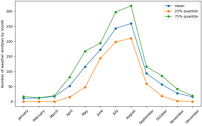
Plotting the monthly statistics

Lastly, we can produce some plots of the stats matrix. First of all, a static plot with some quantiles.

plt.figure(figsize=(8, 5), layout="constrained")
plt.plot(MONTH_NAMES[1:], stats["mean"], "-o", label="mean")
plt.plot(MONTH_NAMES[1:], stats["25%"], "-o", label="25% quantile")
plt.plot(MONTH_NAMES[1:], stats["75%"], "-o", label="75% quantile")
plt.xticks(rotation=45)
plt.ylabel("Number of weather windows by month")
plt.legend()
plt.show()

We can also produce interactive plots to facilitate the visualisation.

fig = go.Figure()
for colname in stats.columns:
    fig.add_trace(
        go.Scatter(
            x=[MONTH_NAMES[i] for i in stats.index],
            y=stats[colname],
            name=colname,
            legendgroup="by_month",
        )
    )

fig.update_xaxes(title_text="Month")
fig.update_yaxes(title_text="Number of Weather Window")
fig.update_layout(
    height=800,
    legend_tracegroupgap=130,
    title="Monthly statistics of number of weather window (Concurrent)",
)
fig

Operational planning

The operational length is how long will it take to carry out the operation of given nominal length, when taking into account weather downtime. Operational length is provided in units of time. When calculating the length, operations can be considered critical or non-critical. With critical operations, the full operations have to restart if criteria is exceeded. With non-critical operations, they can be paused for the bad weather and continued once the conditions meet the criteria.

Operational criteria

criteria = "hs < 1.8 and tp < 9"
oplen = 12
critical_operation = False

Computation of operation durations

Once the criteria are defined, we can proceed to the estimation

oplendetect = oplen_calc(data_matching_criteria, oplen, critical_operation)
results = olmonstats(oplendetect)
stats = (
    results.describe(percentiles=percentiles)
    .drop(["count", "std"])
    .transpose()
    .sort_index()
)

/home/runner/work/py-resourcecode/py-resourcecode/resourcecode/opsplanning/__init__.py:328: FutureWarning:

Series.__getitem__ treating keys as positions is deprecated. In a future version, integer keys will always be treated as labels (consistent with DataFrame behavior). To access a value by position, use `ser.iloc[pos]`

And finally produce visual exploration of the durations.

fig = go.Figure()
for colname in stats.columns:
    fig.add_trace(
        go.Scatter(
            x=[MONTH_NAMES[i] for i in stats.index],
            y=stats[colname],
            name=colname,
            legendgroup="by_month",
        ),
    )

fig.update_xaxes(title_text="Month")
fig.update_yaxes(title_text="Length of operations")
fig.update_layout(
    height=800,
    legend_tracegroupgap=130,
    title="Monthly statistics of length of operations (non-critical operations)",
)
fig