Visualize the database configuration: nodes, bathymetry…

import resourcecode
import numpy as np
import matplotlib.pyplot as plot
import matplotlib.tri as mtri
from mpl_toolkits.axes_grid1.axes_divider import make_axes_locatable

plot.rcParams["figure.dpi"] = 400

Select a node and plot the mesh around

Below is an extract of the nodes locations and characteristics.

resourcecode.data.get_grid_field()

	node	longitude	latitude	depth	d50
0	1	6.922498	62.914669	3.0	0.000
1	2	6.910178	62.913013	3.0	1.322
2	3	6.920552	62.904381	3.0	1.322
3	4	6.933673	62.899376	3.0	1.322
4	5	6.945979	62.900120	3.0	1.322
...	...	...	...	...	...
328025	328026	-4.641320	53.165386	41.0	-1.585
328026	328027	-2.131147	56.025635	67.0	0.737
328027	328028	-5.977029	55.205364	139.0	0.737
328028	328029	-5.939720	55.209774	142.5	-1.585
328029	328030	-4.639367	54.751503	20.0	-1.585

328030 rows × 5 columns

One can also obtain the location of the points where the full 2D spectral data is available using resourcecode.get_grid_spec() function

resourcecode.get_grid_spec()

	longitude	latitude	name	depth	d50
0	1.5000	52.0000	E001500N52000	15.413269	0.737000
1	-5.5000	52.0000	W005500N52000	89.648946	-0.826506
2	-6.0000	52.0000	W006000N52000	95.836144	-1.585000
3	-6.5000	52.0000	W006500N52000	52.674089	0.737000
4	-7.0000	52.0000	W007000N52000	54.674644	0.034650
...	...	...	...	...	...
24271	2.4392	51.3894	WESTHINDER	23.067135	0.364202
24272	3.4155	51.4334	WIELINGENNOORD	8.367460	0.734515
24273	6.0640	53.4100	WIERUMERWAD2	3.000000	1.322000
24274	6.0638	53.4090	WIERUMERWAD3	3.000000	1.322000
24275	4.0084	51.9922	ZDV8-2D-MMND	12.754536	1.099299

24276 rows × 5 columns

Usually, we know the coordinates of the point we want to look at. It is possible to find the closest node from this location, using the following function. It return a vector of dimension two, with the node number and the distance from the requested location (in meters).

# We select the closest node from given coordinates
selected_node = resourcecode.data.get_closest_point(
    latitude=48.3026514, longitude=-4.6861533
)
selected_node

(134940, 296.89)

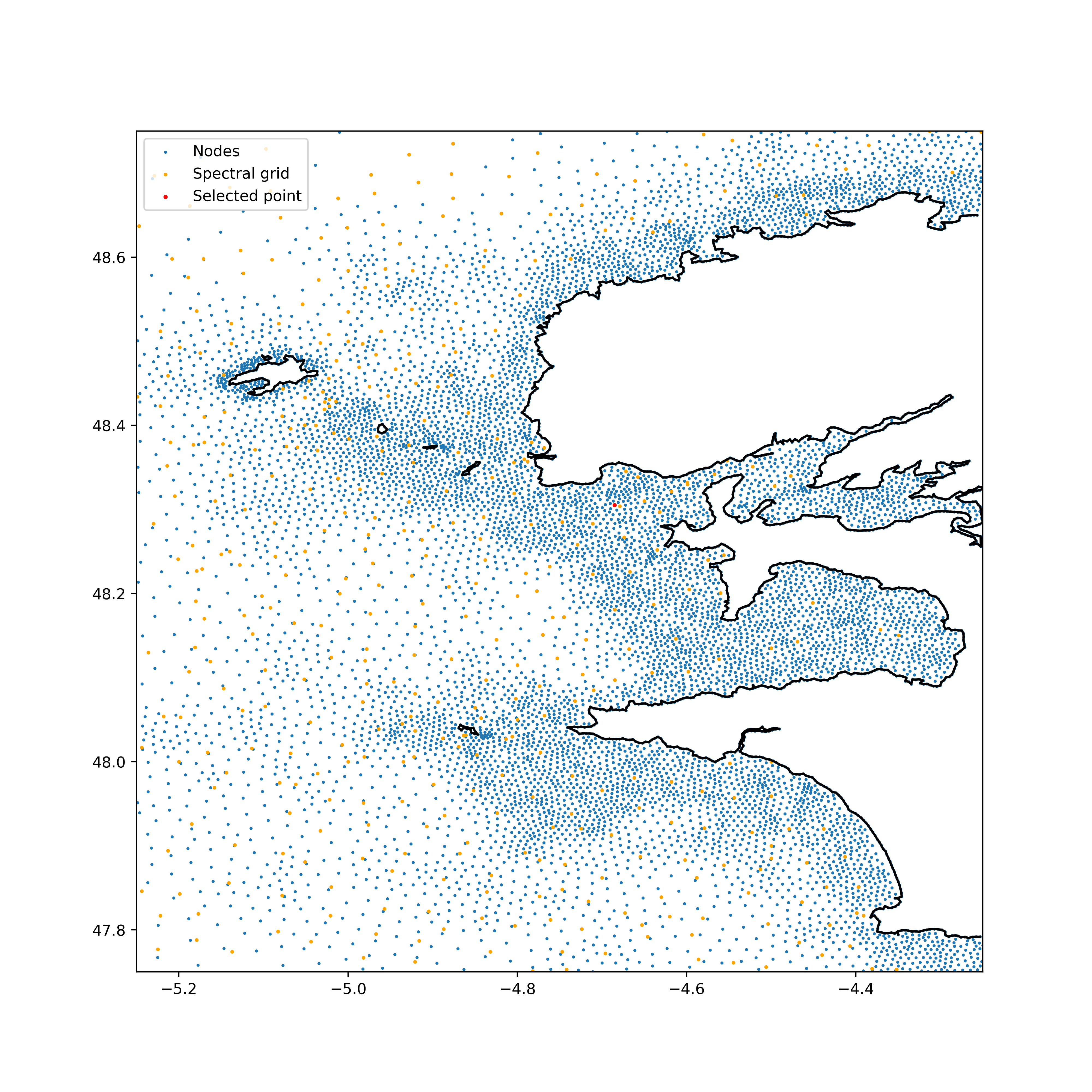
Once the node is selected, it is possible to print a map of the area.

lat_min, lat_max = 47.75, 48.75
lon_min, lon_max = -5.25, -4.25

nodes = resourcecode.data.get_grid_field().query(
    f"latitude <= {lat_max} and latitude >= {lat_min} and longitude > {lon_min} and longitude < {lon_max}"
)
spec = resourcecode.get_grid_spec().query(
    f"latitude <= {lat_max} and latitude >= {lat_min} and longitude > {lon_min} and longitude < {lon_max}"
)
coast = resourcecode.data.get_coastline().query(
    f"latitude <= {lat_max} and latitude >= {lat_min} and longitude > {lon_min} and longitude < {lon_max}"
)
islands = resourcecode.data.get_islands().query(
    f"latitude <= {lat_max} and latitude >= {lat_min} and longitude > {lon_min} and longitude < {lon_max}"
)
plot.figure(figsize=(10, 10))
plot.scatter(nodes.longitude, nodes.latitude, s=1, label="Nodes")
plot.scatter(spec.longitude, spec.latitude, s=2, color="orange", label="Spectral grid")
plot.ylim(lat_min, lat_max)
plot.xlim(lon_min, lon_max)
plot.plot(coast.longitude, coast.latitude, color="black")
classes = list(islands.ID.unique())
for c in classes:
    df2 = islands.loc[islands["ID"] == c]
    plot.plot(df2.longitude, df2.latitude, color="black")
plot.scatter(
    nodes[nodes.node == selected_node[0]].longitude,
    nodes[nodes.node == selected_node[0]].latitude,
    s=3,
    color="red",
    label="Selected point",
)
plot.legend()
plot.show()

---

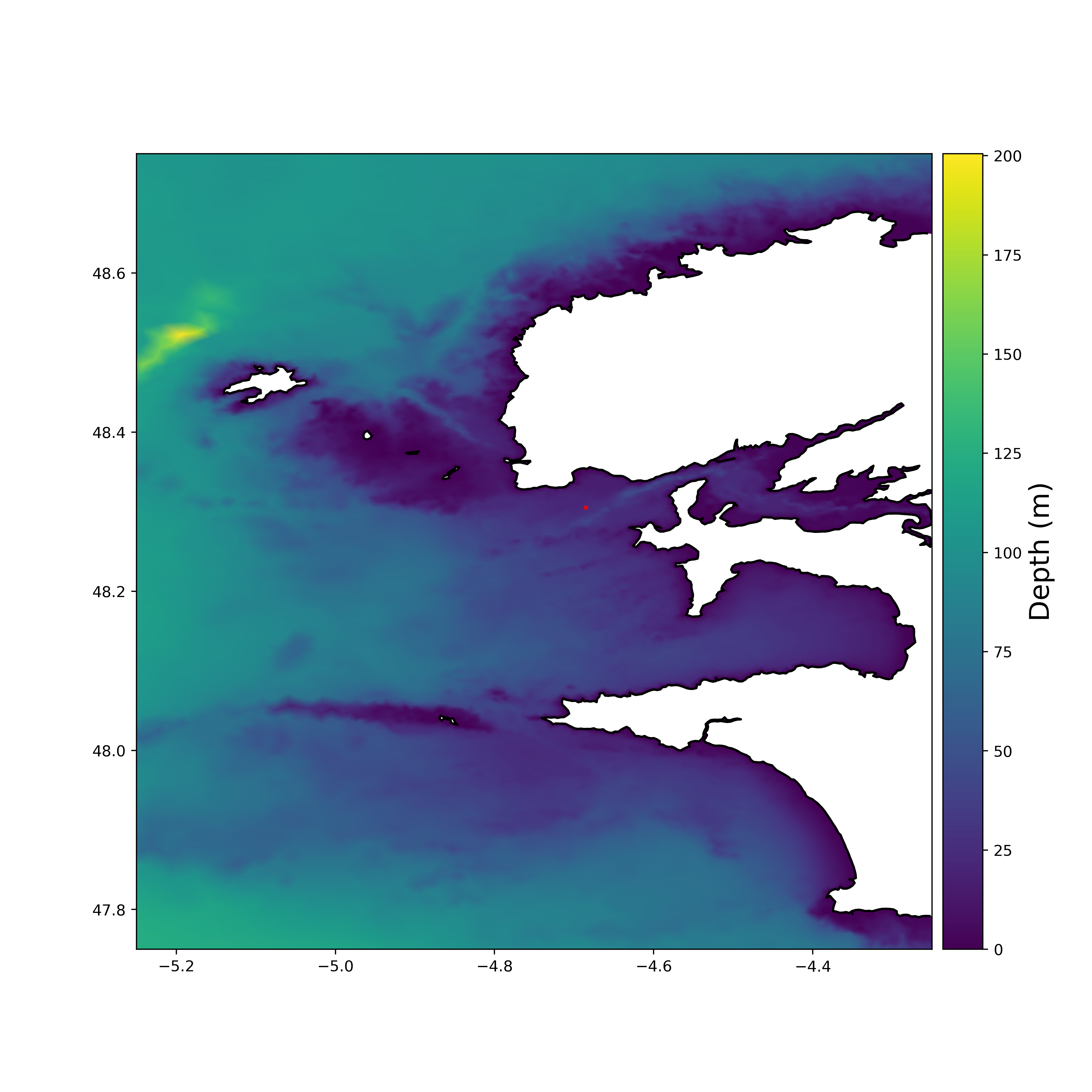
Plot of bathymetry next to the selected point

The data included in the toolbox alows to easily map the depth anywhere on the covered area. The following piece of code shows and example of such a map.

# Importing the data for plotting
tri = (
    resourcecode.get_triangles().to_numpy() - 1
)  # The '-1' is due to the Zero-based numbering of python
field_mesh = resourcecode.data.get_grid_field().to_numpy()
triang = mtri.Triangulation(field_mesh[:, 1], field_mesh[:, 2], tri)

plotted_nodes = (
    (field_mesh[:, 1] <= lon_max)
    & (field_mesh[:, 1] >= lon_min)
    & (field_mesh[:, 2] <= lat_max)
    & (field_mesh[:, 2] >= lat_min)
)

s = field_mesh[:, 3]
s[np.isnan(s)] = 0  # Due to missing values in bathy

fig = plot.figure(figsize=(10, 10))

ax0 = fig.add_subplot(111, aspect="equal")

plot.ylim(lat_min, lat_max)
plot.xlim(lon_min, lon_max)
SC = ax0.tripcolor(triang, s, shading="gouraud")
SC.set_clim(min(s[plotted_nodes]), max(s[plotted_nodes]))
# Plot selected location
plot.scatter(
    nodes[nodes.node == selected_node[0]].longitude,
    nodes[nodes.node == selected_node[0]].latitude,
    s=3,
    color="red",
    label="Selected point",
)
# Add coastlines and islands
plot.plot(coast.longitude, coast.latitude, color="black")
classes = list(islands.ID.unique())
for c in classes:
    df2 = islands.loc[islands["ID"] == c]
    plot.plot(df2.longitude, df2.latitude, color="black")

# Colorbar.
the_divider = make_axes_locatable(ax0)
color_axis = the_divider.append_axes("right", size="5%", pad=0.1)
cbar = plot.colorbar(SC, cax=color_axis)
cbar.set_label("Depth (m)", fontsize=18)
plot.show()